Machine Learning Toolkit (MLT) is a critical app in i2G data analytics workflow. MLT on i2G offers the most advanced predictive algorithms including both regression and classification. It also contains non-linear predictor functions to model non-linear relationship between the input curves and the target curve. Self-organizing Map is another advanced module built specifically for facies classification by both supervised and unsupervised algorithms.

Key values:

o Extraction of meaningful insights from your data and information sources

o Robust algorithms designed by geoscientists and machine learning experts

o Reproducible results by allowing seed number input

o Flexibility in conﬁguring model inputs and architectures

o Easy-to-use and adjustable workflow interface

o Availability of different model validation metrics: offer different ways to assess training and predicting capacity: training/loss error/accuracy cross-plot as well as a confusion matrix

23.1. Overview

· Machine Learning Toolkit on i2G platform is an advanced tool that offers many state-of-the-art algorithms in the industry. They are divided into 2 groups, namely Regression and Classification.

· Fundamentally, classification is about predicting a label (discrete properties such as facies) and regression is about predicting a quantity (continuous properties such as permeability).

· Before running any ML technique, the user is required to create a new ML model.

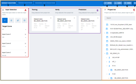
Figure 23‑1 Interface of Machine Learning Toolkit app

The interface of machine learning app contains three main regions: Tool Bar, Working Area (A and B) and Project List (C). The Tool Bar has 7 buttons

Table 23‑1 Buttons in Tool Bar of MLT app

No	Name	Note
1	“DATA SELECTION” tab	Open the tab to select input data, including input curves, target curve and input dataset for training/verify/ prediction
2	“MODEL SELECTION” tab	Open the tab to select machine learning algorithms
3	“TRAINING AND PREDICTION” tab	Open the tab to execute the training, validation and prediction process
4	“OPEN” button	Open other project(s)
5	“SAVE” button	Save the current project(s)
6	“NEW” button	Create a new project(s)
7	Setting button	Open a form for setting the text size

Table 23‑2 Three separate spaces in the working areas

Area	Note
A	Select input curves and the target curve
B	Dataset for training, verification and prediction. These datasets should be dragged and dropped from project data tree on the right (C)
C	List of projects. The user needs to select a dataset, drop them to area B

To build a machine learning model:

Step 1. Go to https://ai.i2g.cloud/

Step 2. Go to DATA SELECTION tab > go to project list > select dataset for getting training, verification and prediction data, then drag and drop them to area B in the middle

Step 3. Go to input selection area A on the left and select one “Target” curve and input curves. The user can select them by curves name , curve family or family group . Users can click on the button ( ) to add input curve.

Step 4. Select MODEL SELECTION tab > Select the type of model under “Type Selection” > configure model architecture by adjusting model parameter

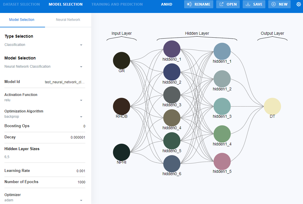
Figure 23‑2 configure model architecture in MLT

Step 5. Select TRAINING AND PREDICTION tab

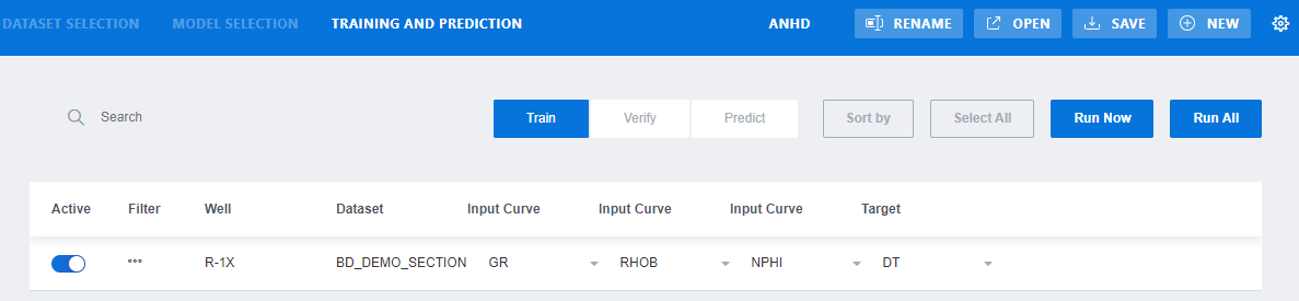
Figure 23‑3 Training and Prediction tab in MLT

Table 23‑3 Buttons in Training and Prediction tab in MLT

Button	Note
Active	Activate/deactivate the selected dataset
Filter	Open a form to discriminate the input data
Input Curve	Select the input curve from the dataset
Train	Tab for configuring training data
Verify	Tab for configuring verifying data
Predict	Tab for configuring prediction data
Run Now	Run the current tab: Train or Verify or Predict
Run All	Run all tabs: Train/Verify/Predict

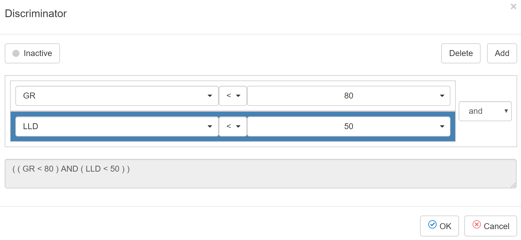
Figure 23‑4 The Discriminator dialog of the Training and Prediction tab in MLT

Table 23‑4 Buttons in Discriminator dialog

Button	Note
Activated/inactive	Select to activate/deactivate the filter
Delete	Delete the selected filter
Add	Add a filter. User can select either AND or OR

To create a filter before training a machine learning model:

Step 1. Select filter icon in front of the dataset

Step 2. Click this icon to set it to “Activated”

Step 3. Select the curve used for discrimination > select the comparison operators > input a value or select a curve to compare to

Step 4. Click OK

23.2. Regression model

23.2.1. Linear regression

This is a linear approach to modelling the relationship between the input variables and output variable. The relationships are modeled using linear predictor functions, so called linear models, whose unknown model parameters are estimated from the data. Like all forms of regression analysis, linear regression focuses on the conditional probability distribution of the outputs given the values of the inputs, rather than on the joint probability distribution of all of these variables, which is the domain of multivariate analysis. All parameters of linear regression model are set as default and will not be changed by the users.

Fit Intercept: (Boolean, default True) this parameter is used to decide whether to calculate the intercept for this model. If set to False, no intercept will be used in calculations (e.g. data is expected to be already centered). In other words, the fitting line for the model is forced to pass the origin (0, 0). If set to True, the line of best fit can "fit" the y-axis. This means the line will not pass the origin.

Normalize: (Boolean, default True) this parameter is ignored when the parameter Fit Intercept is set to False. If True, the inputs X will be normalized to the range (-1, 1) before regression by subtracting the mean and dividing by the standard deviation.

23.2.2. Huber regression

This is a regression method that finds the relationship between inputs and outputs. Basically, that relationship is assumed to be a model, which can be a mapping function, or some mapping rules, connecting the two data. All parameters of the mapping model are ordinarily optimized based on least squared error. This traditional approach will not work well if the dataset is composed of outliers. In order to avoid the effect of outliers, Huber loss function is introduced. Basically, Huber function is a penalty function that is quadratic when the error is small, and is linear if the error is large.

The input parameters are as follows.

Fit Intercept: (Boolean, default True) this parameter is used to decide whether to calculate the intercept for this model. If set to False, no intercept will be used in calculations (i.e. the data is already centered around the origin.). In other words, the fitting curve for the model is forced to pass the origin (0, 0). If set to True, the curve of best fit is allowed not to pass the origin.

Tolerance: (real value, default 0.0001) is a threshold to stop the training process. The iteration will stop if the maximum of projected gradients with respect to all variables of the objective function is smaller than Tol.

Alpha: (real value, default 1) this is the regularize parameter, which is used to avoid overfitting. Increasing the value of alpha results in less overfitting but also greater bias.

Epsilon: (real value greater than 1.0, default 2) this parameter controls the number of samples that should be classified as outliers. The smaller the epsilon, the more robust it is to outliers.

Max Number of Iterations: (integer, default 1000) this parameter determines the maximum number of iterations that the fitting algorithm should run for.

Warm Start: (Boolean, default True) This is useful if the stored attributes of a previously used model has to be reused. If set to False, then the coefficients will be rewritten for every call to fit.

23.2.3. Lasso (least absolute shrinkage and selection operator)

This is a regression analysis method that performs both variable selection and regularization in order to enhance the prediction accuracy and interpretability of the statistical model it produces.

The input parameters for this model are as follows.

Random State: (integer) this parameter determines the seed of the pseudo random number generator that selects a random feature to update.

Max Number of Iteration: (integer, default 1000) this is the maximum number of iterations that the training process goes through.

Alpha: (real value, default 1) this is the coefficient determining the relationship between output errors and the variance of the inputs. Alpha = 0 is equivalent to an ordinary least square, solved by the Linear Regression object. For numerical reasons, using Alpha = 0 with the Lasso object is not advised. Given this, you should use the Linear Regression object.

Tolerance: (real value, default 0.0001) is the tolerance for the optimization: if the updates are smaller than tolerance, the optimization code checks the dual gap for optimality and continues until it is smaller than Tolerance value.

23.2.4. Decision tree

This is a prediction model that uses a tree-like graph of decisions and their possible consequences, including chance event outcomes, resource costs, and utility. It breaks down a dataset into smaller and smaller subsets while at the same time an associated decision tree is incrementally developed. The final result is a tree with decision nodes and leaf nodes. A decision node has two or more branches representing values for the attribute tested. Each leaf node represents a decision on the numerical target. The topmost decision node in a tree which corresponds to the best predictor is called root node.

Input parameters for this model are as follows.

Max Depth of Trees: (integer, default 3) this parameter determines the maximum depth of the tree. If “0”, then nodes are expanded until all leaves are pure or until all leaves contain less than min_samples_split samples.

Max Features: (integer, default 1) this is the number of features to consider when looking for the best split.

Ranking Criterion: (integer, default “mse”) The function to measure the quality of a split. Supported criteria are “mse” for the mean squared error, which is equal to variance reduction as feature selection criterion and minimizes the L2 loss using the mean of each terminal node, “friedman_mse”, which uses mean squared error with Friedman’s improvement score for potential splits, and “mae” for the mean absolute error, which minimizes the L1 loss using the median of each terminal node.

Random State: (integer) this is the seed used by the random number generator.

Splitter: (default “random”) The strategy used to choose the split at each node. Supported strategies are “best” to choose the best split and “random” to choose the best random split.

23.2.5. Random forest

This is a regression method that constructs a multiple of decision trees at training time and outputs the mean prediction of the individual trees. This approach overcomes the overfitting behavior of single decision trees. The collection of decision trees is generated such that each individual tree is uncorrelated with the others by using different bootstrapped samples from the training data.

The input parameters of the random forest regressor are as follows.

Number of Estimators: (integer, default 150) is the number of trees in the forest.

Max Depth: (integer, default 1) is the maximum depth of the tree. If “0”, then nodes are expanded until all leaves are pure.

Max Features: the number of input features is used when looking for the best split. The value of this parameter is the same as in Decision tree.

Boostrap: (Boolean, default True) to determine whether bootstrap samples are used when building trees. If False, the whole dataset is used to build each tree.

Ranking Criterion: (default “mse”) The function to measure the quality of a split. Supported criteria are “mse” for the mean squared error, which is equal to variance reduction as feature selection criterion, and “mae” for the mean absolute error.

Random State: is the seed used by the random number generator.

23.2.6. XG Boost

XGBoost stands for extreme gradient boosting method, which is used for supervised learning problems, where we use the training data (with multiple features) xi to predict a target variable yi. is an efficient and scalable implementation of gradient boosting algorithm. Function estimation is inspected from the aspect of numerical optimization in function space, rather than parameter space. This is a more regularized model formalization to control over-fitting, which gives it better performance than traditional gradient boosting method.

Input parameters of this model are as follow.

Number of Estimators: (integer, default 150) number of trees created.

Max Depth: (integer, default 5) Maximum depth of a tree. Increasing this value will make the model more complex and more likely to overfit. Beware that XGBoost aggressively consumes memory when training a deep tree.

Gamma: (default 0.5) Minimum loss reduction required to make a further partition on a leaf node of the tree. The larger gamma is, the more conservative the algorithm will be. Range [0, ꝏ].

Booster: (Default “gbtree”) Which booster to use. Can be gbtree, gblinear or dart; gbtree and dart use tree based models while gblinear uses linear functions.

Regularization alpha: (integer, default 1) L1 regularization term on weights. Increasing this value will make model more conservative.

Regularization lambda: (integer, default 1) L2 regularization term on weights. Increasing this value will make model more conservative.

Random State: is the seed used by the random number generator.

23.2.7. Support vector machine (SVM Regression)

Support vector machine for regression works in a way that is almost the same as for classification problems, except that the maxima margin is added by a tolerance factor epsilon, which is set in approximation to the SVM such that it can adapt to the real input values. Input parameters of SVM regression model are as follows.

Kernel: (default “rbf”) name of kernel function

C: (default 2) this is the parameter for the soft margin cost function, which controls the influence of each individual support vector. A large C gives you low bias and high variance, which means you penalize the cost of error a lot. A small C gives you higher bias and lower variance, which means higher generalization.

Gamma: (default 0.1) kernel parameter for ‘rbf’, ‘poly’ and ‘sigmoid’. This parameter can affect the data transformation behavior. Intuitively, a small gamma value means two points can be considered similar even if are far from each other. In the other hand, a large gamma value means two points are considered similar just if they are close to each other. So a small gamma will give you low bias and high variance while a large gamma will give you higher bias and low variance.

Degree: (default 2) is the degree of the polynomial kernel function (‘poly’). Ignored by all other kernels.

Tolerance: (default 0.001) Tolerance for stopping criterion..

Max Number of Iterations: (default 100) Hard limit on iterations within solver, or -1 for no limit.

23.2.8. Neural Network Regression

It is a class of feedforward artificial neural network. A neural network consists of three types of layers of nodes, including input layer, hidden layers, and output layer. Except for the input nodes, each of other nodes is a neuron that uses a nonlinear activation function. NN can be used for both classification and regression problems. The supervised learning technique utilized for NN is backpropagation algorithm. Input parameters for this model are defined as follows.

Solver: (default “lbfgs”) The solver for weight optimization.

· ‘lbfgs’ is an optimizer in the family of quasi-Newton methods.

· ‘sgd’ refers to stochastic gradient descent.

· ‘adam’ refers to a stochastic gradient-based optimizer proposed by Kingma, Diederik, and Jimmy Ba

· ‘Cg’ is the conjugate-gradient optimization algorithm. Apart from the well-known backpropagation algorithm, users can also use Conjugate Gradient as a training algorithm for Neural networks. All input parameters for conjugate gradient neural network have the same meaning as those in MLP.

Note: The default solver ‘adam’ works pretty well on relatively large datasets (with thousands of training samples or more) in terms of both training time and validation score. For small datasets, however, ‘lbfgs’ can converge faster and perform better.

Activation Function: (default “relu”) is the name of activation function for hidden nodes.

· ‘identity’, no-op activation, useful to implement linear bottleneck, returns f(x) = x

· ‘logistic’, the logistic sigmoid function, returns f(x) = 1 / (1 + exp(-x)).

· ‘tanh’, the hyperbolic tan function, returns f(x) = tanh(x).

· ‘relu’, the rectified linear unit function, returns f(x) = max(0, x)

Max number of iterations: (integer, default 500) is the maximum number of iterations. The solver iterates until convergence (determined by the parameter ‘tolerance’) or this number of iterations. For stochastic solvers (‘sgd’, ‘adam’), note that this determines the number of epochs (how many times each data point will be used), not the number of gradient steps.

Tolerance: (default 0.0003) Tolerance for the optimization. When the loss or score is not improving by at least Tol for two consecutive iterations, convergence is considered to be reached and training stops.

Learning rate initialization: (default 0.001) It controls the step-size in updating the weights. Only used when solver is ’sgd’ or ‘adam’.

23.3. Classification model

23.3.1. Decision Tree

This is a non-parametric supervised learning method used for classification or regression. The goal is to create a model that predicts the value of a target variable by learning simple decision rules inferred from the data features. The decision tree is built by recursively selecting the best attribute to split the data and expanding the leaf nodes of the tree until the stopping cirterion is met. The choice of best split test condition is determined by comparing the impurity of child nodes and also depends on which impurity measurement is used. If the decision trees are too large, overfitting may occur. Input parameters for decision tree classifiers are defined as follows.

Ranking Criterion: (default “entropy”) is the function to measure the quality of split.

· “gini”: is for the Gini impurity. This is a measure of how often a randomly chosen element from the set would be incorrectly labeled if it was randomly labeled according to the distribution of labels in the subset. It reaches its minimum (zero) when all cases in the node fall into a single target category.

· “entropy”: is for the information gain. Information gain is used to decide which feature to split on at each step in building the tree. In order to keep the tree small, at each step we should choose the split that results in the purest daughter nodes, which correspond to the feature with highest information gain with the output labels. The split with the highest information gain will be taken as the first split and the process will continue until all children nodes are pure, or until the information gain is 0.

Min samples split: (integer, default 5) is the minimum number of samples required to split an internal node. The larger the min_samples is, the bigger trees can be created.

Min Impurity Decreases: (Real values, default 0.01) is the threshold for early stopping in tree growth. A node will split if its impurity is above the threshold, otherwise it is a leaf. This value will also determine the size of trees.

23.3.2. Nearest neighbors (KNN)

This is a non-parametric method used for classification. The input consists of the k closest training examples in the feature space. The output is a class membership. An object is classified by a majority vote of its neighbors, with the object being assigned to the class most common among its K nearest neighbors (K is a positive integer, typically small). If K = 1, then the object is simply assigned to the class of that single nearest neighbor. Input parameters for this model is defined as follows.

Number of Neighbors: (default 100) is the number of closest training samples to the testing sample.

P: (default 1) is the power parameter for the Minkowski metric. It determines how to calculate the distance between samples. When p = 1, this is equivalent to using manhattan_distance (l1), and euclidean_distance (l2) for p = 2. For arbitrary p, minkowski_distance (l_p) is used.

Distance Metric: (minkowski distance) determines the method to calculate the distance between samples

23.3.3. Logistic Regression

This classification algorithm is named for the function used at the core of the method, the logistic function. The logistic function, also called the sigmoid function is an S-shaped curve that can take any real-valued number and map it into a value between 0 and 1, but never exactly at those limits. f = 1 / (1 + e^-value), where e is the base of the natural logarithms. There can be many different equations used for logistic regression, for example: y = e^(b0 + b1*x) / (1 + e^(b0 + b1*x)), where y is the predicted output, b0 is the bias or intercept term and b1 is the coefficient for the single input value (x). Each column in your input data has an associated b coefficient (a constant real value) that must be learned from your training data.

Logistic regression is a linear method, but the predictions are transformed using the logistic function. The impact of this is that we can no longer understand the predictions as a linear combination of the inputs as we can with linear regression.

Logistic regression models the probability of the default class. In this model we use 30 logistic regression classifiers corresponding to 30 different default classes. For each classifier, the default class is fitted against all the other classes, resulting in the probability of the data sample being 1 of the 30 classes. In the prediction phase, the class with the highest output probability will be assigned to the testing sample.

The setting parameters for this model are described as follows.

C: (default 20) is the inverse of regularization strength. Like in support vector machines, smaller values specify stronger regularization.

Max Number of Iterations: (default 10000) Maximum number of iterations taken for the solvers to converge.

Solver: (default “liblinear”) is the name of the algorithm to use in the optimization problem.

23.3.4. Random Forest

A random forest is a meta estimator that fits a number of decision tree classifiers on various sub-samples of the dataset and use averaging to improve the predictive accuracy and control over-fitting. The sub-sample size is always the same as the original input sample size but the samples are drawn with replacement if bootstrap=True (default).

Input parameters for this method are defined as follows.

Number of Trees: (default 150) The number of decision trees in the forest

Ranking Criterion: (default “entropy”) The function to measure the quality of a split. This is the same as in decision tree.

Min Samples Split: (default 5) The minimum number of samples required to split an internal node. This is the same as in decision tree.

Min Impurity Decrease: (default 0.0003) Threshold for early stopping in tree growth. This is the same as in decision tree.

23.3.5. Neural network

This is a multilayer perceptron network for classification problem. This model optimizes the log-loss function using LBFGS or stochastic gradient descent. Input parameters for this model are defined as follows.

Activation Function: (default “relu”) is the name of activation function for hidden layers.

Optimization Algorithm: (default “backprop”) is the name of training algorithm, which is either backpropagation or evolution strategy algorithm.

Backpropagation algorithm works best with a large number of epochs.

Evolution algorithm is preferable with smaller number of epochs, about 1000.

Learning Rate: (default 0.001) It controls the step-size in updating the weights.

Number of Epochs: (default 1000) maximum number of training iterations.

Optimizer: (default “adam”) is the solver for weight optimization.

Warm up: (default “false”) is to determine the initial values of weights. When set to True, the model will run with batch_size = 1 and num_epochs = 1 to get the initial weights, otherwise, it just randomizes the initial weights. After this process, the model will run the training process as set by other parameters.

Boosting Ops: (default 0) this parameter is only used for evolution algorithm. This parameter determines the number of times that the weights are further updated based on the accuracy after the training process based on the loss function finishes. Default is 100.

Sigma: (default 0.01) this parameter is only used for evolution algorithm. This parameter determines the variance size of the Gaussian distribution used for randomizing the weights.

Population: (default 50) is the number of sets of randomized weights for each epoch. This parameter is only used for evolution algorithm.

Decay: (default 0.000001) is to determine the decaying rate of weight updates.

23.4. Self-organizing Map (SOM)

Self-Organizing Maps (SOMs) is a type of artificial neural network that is trained using unsupervised learning to produce a low-dimensional (typically two-dimensional), discretized representation of the input space of the training samples, called a map, and is therefore a method to do dimensionality reduction. Self-organizing maps apply competitive learning in the sense that they use a neighborhood function to preserve the topological properties of the input space. This makes SOMs useful for visualization by creating low-dimensional views of high-dimensional data.

SOM can provide an interpretation of the dataset about data distribution, the number of clusters and some other visualizations. Thus, SOM is traditionally considered as both a dimensional reduction tool and a clustering tool. It has been shown that while self-organizing maps with a small number of nodes behave in a way that is similar to the K-means algorithm, larger self-organizing maps rearrange data in a way that is fundamentally topological in character.

In general, the weights of the neurons are initialized either to small random values, or by randomly choosing samples from the training data to initialize the weights of neurons, or sampled evenly on the plane formed by the two largest principal component eigenvectors.

The self-organizing system in SOM is a set of nodes (or neurons) connected to each other via a topology of rectangle. This set of nodes is called a map. Each neuron has several nearest neighbors (4 or 8 with rectangular topology). At each training step, an input vector Xi is introduced to the map, using the Euclidean distance, the different between Xi and each neuron in the map is calculated. The most similar neuron to the selected sample is called the winning node or the best-matching unit (BMU). The weight vector of the BMU is then updated by a learning rule:

W_i (t+1)= W_i (t)+ θ(t).α(t).(X_i - W_i (t))

Where W_i (t+1) is the newly updated weight vector of BMU at time t+1. α(t) is the learning rate which decreases over each training iteration. By this learning rule, the BMU is moved closer to the chosen input vector. Instead of applying the winner-takes-all principal, the BMU’s neighboring neurons can also be updated. The neighborhood of BMU is determined by BMU’s radius. The learning rate of BMU, α(t), is decaying after each updating iteration as follows:

α(t)=α_0/(1+ decay_rate *t)

Where, t is the maximum number of update iterations; α_0 is the initial learning rate.

θ(t) is the neighboring index determining how much a neighboring neuron is updated in each iteration. Depending on different neighboring methods, θ(t) can be calculated differently as:

· Bubble method: all neurons inside the distance from the BMU will be updated.

θ(t)={■(1 if dist≤σ(t)@0 if dist>σ(t))┤

Where, σ(t) is the distance function between BMU and other neurons, which also decays during the update process.

· Gaussian method: all neurons will be updated with the distance index defined as

θ(t)=e^(-〖dist〗^2/(2〖σ(t)〗^2 ))

Where, “dist” is the Euclidean distance between the BMU and other neurons.

tIn those methods, The distance function σ(t) is defined as

σ(t)=σ_0/(1+sigma_decay_rate *t)

Where σ_0 is the initial neighboring radius, and the sigma_decay_rate determines how much the distance function decays after each iteration.

23.4.1. Unsupervised SOM (Clustering model)

This is a traditional use of the SOM as discussed above. The input data samples are clustered using SOM. Users can manage following parameters:

Number of Columns: (integer, default 10) This is the number of columns of neurons in the topology of rectangle of the SOM.

Number of Rows: (integer, default 10) This is the number of rows of neurons in the topology of rectangle of the SOM.

Random State: (integer) this is the seed used by the random number generator.

Learning Decay Rate: (real) is the decay_rate.

Learning Rate: (real, in range (0, 1)) is the initial learning rate α_0.

Neighborhood: (bubble or Gaussian) is the method to determine the neighboring index θ(t).

Weight Initialization: (random, sample, or PCA) is the method to initialize the weights of all neurons in the SOM.

Random: the weights are generated as small random values,

Sample: the weights are generated by randomly choosing samples from the training data

PCA: the weights are sampled evenly on the plane formed by the two largest principal component eigenvectors of the training data.

Sigma: (real) is the initial neighboring radius, σ_0.

Sigma Decay Rate: (real) is the rate for the neighboring radius to decay over updating iterations.

Batch Size: (integer) is the number of samples in the same batch during learning phase.

Number of Clusters: (integer) is the number of clusters that users want to divide the data using SOM.

23.4.2. Supervised SOM (Classification model)

This is a combination method between the traditional SOM and the Learning Vector Quantization (LVQ) algorithm to form a classification version of SOM. SOM will be supervised trained using labeled training data to create a classification model.

The supervised training process for SSOM includes two phases as depicted in the below figure

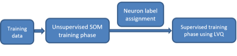
Figure 23‑5 Two phases of the supervised training process for SSOM

Unsupervised SOM training phase follows traditional SOM algorithm. The input training dataset is used to generate the clustering model of the SOM.

After the first phase, all neurons in the SOM are labeled based on the closest training samples.

Supervised training phase is based on LVQ algorithm, which moves the labeled neurons closer to the training samples having the same labels, or moves the neurons further to the sample having different labels.

Users can manage following parameters:

Number of Columns: (integer, default 10) This is the number of columns of neurons in the topology of rectangle of the SOM.

Number of Rows: (integer, default 10) This is the number of rows of neurons in the topology of rectangle of the SOM.

Random State: (integer) this is the seed used by the random number generator.

Learning Decay Rate: (real) is the decay_rate.

Learning Rate: (real, in range (0, 1)) is the initial learning rate α_0.

Neighborhood: (bubble or Gaussian) is the method to determine the neighboring index θ(t).

Weight Initialization: (random, sample, or PCA) is the method to initialize the weights of all neurons in the SOM.

Random: the weights are generated as small random values,

Sample: the weights are generated by randomly choosing samples from the training data

PCA: the weights are sampled evenly on the plane formed by the two largest principal component eigenvectors of the training data.

Sigma: (real) is the initial neighboring radius, σ_0.

Sigma Decay Rate: (real) is the rate for the neighboring radius to decay over updating iterations.

Sup Batch Size: (integer) is the number of samples in the same batch during supervised learning phase.

Sup Number of Iterations: (integer) is maximum number of supervised training iterations.

Sup Batch Size: (integer) is the number of samples in the same batch during supervised learning phase.

Sup Number of Iterations: (integer) is maximum number of supervised training iterations.

Unsup Batch Size: (integer) is the number of samples in the same batch during unsupervised learning phase.

Unsup Number of Iterations: (integer) is maximum number of unsupervised training iterations.

23.4.3. Distributed Ensemble SOM (Advanced Classification SOM)

This is an improved classification model based on supervised SOM. In this model, multiple SOM ensembles are generated based on multiple subsets of input features. Each feature subset is selected either by random or by weighting method. One feature subset is used to create a classification SOM model. Since the size of feature subset is much smaller than the original feature set, the complexity of each ensemble SOM structure can be reduced. Moreover, if the original data is divided into multiple subsets with different feature sets, the information of the training data can be closer analyzed under different angles. This results in a better performance of the classification algorithm. Also, the combination of multiple ensemble SOM may help reduce the variance of the classification errors. From a set of local decisions provided my multiple ensemble SOMs, the test sample is assigned a label based on the majority voting rule.

In this method, the training feature set is divided into multiple feature subset. This looks like a system managed by multiple distributed sensors, each of which contributes a different set of measurements. The name of this method is motivated from this implication.

In this method, users can manage following parameters:

Number of Estimator: (integer, default 30) is the number of ensemble SOMs created in the algorithm.

Random State: (integer) this is the seed used by the random number generator.

Size of Estimator: (integer, default 4) is the size of the ensemble SOMs with a square topology. Here, “Size” is the number of rows as well as the number of columns of each ensemble SOM.

Learning Decay Rate: (real) is the decay_rate.

Learning Rate: (real) is the initial learning rate α_0.

Neighborhood: (bubble or Gaussian) is the method to determine the neighboring index θ(t).

Sigma: (real) is the initial neighboring radius, σ_0.

Sigma Decay Rate: (real) is the rate for the neighboring radius to decay over updating iterations.

Sup Batch Size: (integer) is the number of samples in the same batch during supervised learning phase.

Sup Number of Iterations: (integer) is maximum number of supervised training iterations.

Subset Size: (real, in the range (0, 1]) is the size of training data selected for SOM learning processes.

Sup Number of Iterations: (integer) is maximum number of supervised training iterations.

Unsup Batch Size: (integer) is the number of samples in the same batch during unsupervised learning phase.

Unsup Number of Iterations: (integer) is maximum number of unsupervised training iterations.

Feature Selection: (random or weights) is the method to generate feature subsets

Random: each feature subset is generated by uniformly selection from a pool of original feature set.

Weights: the features are first assigned weights according to their correlation coefficients with the labels. Each feature set is made from a weighted selection from the original feature set. Features with higher weights tend to be selected more often into feature subsets than the ones with smaller weights.

23.4.4. Ensemble Boosting SOM (Advanced Classification SOM)

Motivated from boosting algorithm using multiple ensembles. This approach aims at creating multiple simple SOM models, each of which is created from a subset of training data. In general, each training subset is randomly selected from the training dataset. Each training subset is used to train a supervised SOM model. Decisions from multiple SOMs will be fused based on the majority voting rule. This approach may produce a better performance than single supervised SOM model since it helps reduce the variance of the classification errors.

In this method, users can manage following parameters:

Number of Estimator: (integer, default 50) is the number of ensemble SOMs created in the algorithm.

Random State: (integer) this is the seed used by the random number generator.

Size of Estimator: (integer, default 4) is the size of the ensemble SOMs with a square topology. Here, “Size” is the number of rows as well as the number of columns of each ensemble SOM.

Weight Initialization: (random, sample, or PCA) is the method to initialize the weights of all neurons in the SOM.

Random: the weights are generated as small random values,

Sample: the weights are generated by randomly choosing samples from the training data

PCA: the weights are sampled evenly on the plane formed by the two largest principal component eigenvectors of the training data.

Learning Decay Rate: (real) is the decay_rate of the learning rate.

Learning Rate: (real) is the initial learning rate α_0.

Neighborhood: (bubble or Gaussian) is the method to determine the neighboring index θ(t).

Sigma: (real) is the initial neighboring radius, σ_0.

Sigma Decay Rate: (real) is the rate for the neighboring radius to decay over updating iterations.

Sup Batch Size: (integer) is the number of samples in the same batch during supervised learning phase.

Sup Number of Iterations: (integer) is maximum number of supervised training iterations.

Subset Size: (real, in the range (0, 1]) is the size of training data selected for SOM learning processes.

Sup Number of Iterations: (integer) is maximum number of supervised training iterations.

Unsup Batch Size: (integer) is the number of samples in the same batch during unsupervised learning phase.

Unsup Number of Iterations: (integer) is maximum number of unsupervised training iterations.

23.5. Non-linear Regression

This is a nonlinear approach to model the relationship between the input curves and the target curve. The relationships are modeled using nonlinear predictor functions, so called nonlinear models, whose unknown model parameters are estimated from the data. The nonlinear relationship function is defined by the user, where the variables x1, x2, … correspond to the input curves from top to bottom, respectively.

Table 23‑5 Guides to input nonlinear functions

Algebra expression	Input Syntax	Meaning
a . x	a*x	a multiplied by x
a : x	a/x	a divided by x
a + x	a+x	a plus x
a - x	a-x	a minus x
	a**x	a power x
Ln(x)	log(x)	Natural logarithm of x
Log(x)	log(x)/log(10)	Base 10 logarithm of x
Log_a(x)	log(x)/log(a)	Base a logarithm of x
e	e	Natural number (2.71828). No other parameter named e is permitted.